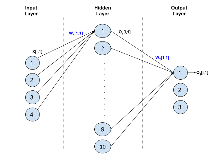
In this post I attempt to describe the calculus involved in backpropogating gradients for the Softmax layer of a neural network. I will use a sample network with the following architecture (this is same as the toy neural-net trained in CS231n’s Winter 2016 Session, Assignment 1). This is a fully-connected network - the output of each node in Layer t goes as input into each node in Layer t+1.
The Forward Pass
Input Layer: Each training example consists of four features. If we have five training examples, then the entire training set input can be represented by the following matrix, each row of which corresponds to one training example:
\[X = \left( \begin{array}{ccc} x_{1,1} & \ldots & \ x_{1,4}\\ \vdots & \vdots & \vdots \\ x_{5,1} & \ldots & \ x_{5,4}\\ \end{array} \right)\]Hidden Layer: For the ith training example, X[i,:], the jth node in this hidden layer will first calculate the weighted sum of the four feature inputs and add some bias to the weighted sum, to calculate what is called Z1[i,j]. It will then apply the layer’s activation function on Z1[i,j] to calculate the output O1[i,j].
This operation will implemented by the following matrix operations.
\[\mathrm{Z_1 = XW_1 + b_1}\] \[\mathrm{O_1 = f(Z_1)}\]where, the weight and bias matrices look like the following:
\[W_1 = \left( \begin{array}{ccc} w_{1,1} & \ldots & \ w_{1,10}\\ \vdots & \vdots & \vdots \\ w_{4,1} & \ldots & \ w_{4,10}\\ \end{array} \right)\]and
\[b_1 = \left( \begin{array}{c} b_{1}, & \ldots, & \ b_{10}\\ \end{array} \right)\]Output Layer: This is the Softmax layer. For ith training example, the kth node in this output layer will first calculate a score, S[i,k], which is a weighted sum of the ten inputs it receives from the Hidden layer.
\[\mathrm{S[i,k] = \sum_{p=1}^{10} {(O_1[i,p] \times W_2[p,k])} + b_2[k]}\]In matrix form:
\[\mathrm{S = O_1W_2 + b_2}\]The kth node will then calculate the un-normalized probability, U[i,k]
\[\mathrm{U[i,k] = e^{S[i,k]}}\]Lastly, the kth node will calculate the normalized probability O2[i,k]
\[\mathrm{O_2[i,k] = \frac{U[i,k]}{\sum_{p=1}^3 U[i,p]}}\]The Loss Function
The contribution of ith training example to network’s loss, Li is:
\[L_i = -\log O_2[i, y_i]\]where yi is the correct label for the ith example. The total loss L is:
\[L = \sum_{i=0}^5 L_i\]Backpropogation
Here I will only attempt to explain ‘backpropogation of the Softmax layer’, i.e., I’m interested in figuring out the impact of tweaking W2 and b2 on the total loss L. Also note that for the sake of simplifying presentation, I have not added any regularization terms to L.
We are interested in measuring the impact of slightly tweaking the weight W2[m,n] on L. This is measured by the following derivative expression:
\[\frac{dL}{dW_2[m,n]} = \sum_{i=1}^5 \frac{dL_i}{dW_2[m,n]}\]We will use the multivariate chain rule to compute this expression.
\[\frac{dL_i}{dW_2[m,n]} = \sum_{k=1}^3 {\underbrace{\frac{\partial L_i}{\partial S[i,k]}}_{\text{Exp. 1}}\times \underbrace{\frac{dS[i,k]}{dW_2[m,n]}}_{\text{Exp. 2}}} \tag{Gradient Equation}\]Solving for Expression 1,
\[\frac{\partial L_i}{\partial S[i,k]} = \frac{\partial L_i}{\partial O_2[i,y_i]} \times \frac{\partial O_2[i,y_i]}{\partial S[i,k]} \tag{1}\] \[\frac{\partial L_i}{\partial O_2[i,y_i]} = \frac{-1}{O_2[i,y_i]} \tag{1.1}\]Intuition for Eq. 1.1: If the normalized ‘probability’ (given by \(O_2[i, y_i]\)) for the correct class yi is small (ideally we want it to be close to 1), then we see from Eq. 1.1 that the gradient of Li w.r.t \(O_2[i, y_i]\) is a large negative number. This implies that any tweak to the network’s parameters which increases the normalized ‘probability’ for the correct class \(y_i\) by a small bit should drive a relatively large decline in the loss \(L_i\).
If \(k = y_i\),
\[\begin{align} \frac{\partial O_2[i,y_i]}{\partial S[i,k]} &= \frac{U[i,k]}{\sum_{p=1}^3 U[i,p]} - \frac{U[i,k]^2}{(\sum_{p=1}^3 U[i,p])^2} \\ \\ &= O_2[i,k] \times (1 - O_2[i,k]) \tag{1.2.1} \end{align}\]If \(k \ne y_i\),
\[\begin{align} \frac{\partial O_2[i,y_i]}{\partial S[i,k]} &= U[i,y_i] \times \frac{-1}{\sum_{p=1}^3 U[i,p]^2} \times U[i,k] \\ \\ &= -O_2[i,y_i] \times O_2[i,k] \tag{1.2.2} \end{align}\]Combining the results of equations \(1\), \(1.1\), \(1.2.1\), and \(1.2.2\), we get:
\[\frac{\partial L_i}{\partial S[i,k]} = \tag{1.3} \begin{cases} (O_2[i,k] - 1), & \text{if k = y_i} \\[2ex] O_2[i,k], & \text{if k $\ne$ y_i} \end{cases}\]Solving for Expression 2,
\[\frac{dS[i,k]}{dW_2[m,n]} = \begin{cases} O_1[i,m], & \text{if k = n} \\[2ex] 0, & \text{if k $\ne$ n} \end{cases}\]Now that we have evaluated Expression 1 and Expression 2, we can see by looking at the Gradient Equation that the summation over three values of \(k\) will be zero \(\forall k \ne n\) (because Exp. 2 is non-zero only for \(k = n\)). We can now write the Gradient Equation as:
\[\frac{dL_i}{dW_2[m,n]} = \begin{cases} (O_2[i,n] - 1) \times O_1[i,m], & \text{if y_i = n} \\[2ex] O_2[i,n] \times O_1[i,m], & \text{if y_i $\ne$ n} \end{cases}\]It is easy to write a vectorized implementation in Python to calculate gradients of \(L\) w.r.t. \(W_2\) (the snippet below assumes \(O_1\) & \(O_2\) have already been calculated):
dL_by_dS = O_2
dL_by_dS[np.arange(5), y] -= 1
dL_by_dW2 = (-1.0/5)*np.matmul(O_1.T, dL_by_dS)