In this post I will attempt to describe the calculus required for a backward pass through a Batch Normalization layer of a Neural Network. For the sake of simplifying presentation, I will assume that we are working with inputs which have a single feature, i.e. xi which is the input vector into the BatchNorm layer, has a single element.

Preliminaries

The BatchNorm layer makes the following adjustments to its input:

Normalization: Assume there are N training examples in the batch we are using for forward and backward passes. The BatchNorm layer first estimates the mean and variance statistics of the batch:

\[(Mean) \space \mu = \frac {1}{N} {\sum_{j=1}^N {x_j}}\] \[(Variance) \space \sigma^2 = \frac {1}{N} \sum_{j=1}^N{(x_j - \mu)^2}\]

It then calculates the “normalized” version of each training example xi:

\[\hat {x_i} = \frac {(x_i - \mu)}{\sqrt {(\sigma^2 + \epsilon)}}\]

Shifting & Scaling: The layer multiplies the normalized input by a “scaling” factor and then adds a “shift”:

\[y_i = \gamma\hat {x_i} + \beta\]

The Backward Pass

The layer receives as input, the gradient of the loss function w.r.t. the outputs of the layer. If L denotes the loss function, then the layer receives as input:

\[\mathrm{ \left( \begin{array}{c} {\frac{\partial L}{\partial y_{1}}}, & \ldots, & {\frac{\partial L}{\partial y_{N}}}\\ \end{array} \right) }\]

We want to compute these quantities, out of which I will focus on the first one for this blog post:

\[\left( \begin{array}{c} {\frac{\partial L}{\partial x_{1}}}, & \ldots, & {\frac{\partial L}{\partial x_{N}}}\\ \end{array} \right)\] \[\frac{\partial L}{\partial \gamma}\] \[\frac{\partial L}{\partial \beta}\]

Using the multivariate chain rule, we get the following expression for our gradient (i refers to the ith training example):

\[\frac {\partial L}{\partial x_i} = \sum_{k=1}^N \left( {\underbrace{\frac{\partial L}{\partial y_k}}_{\text{Exp. 1}} \times \underbrace{\frac {\partial y_k}{\partial x_i}}_{\text{Exp. 2}}} \right) \tag{Gradient}\]

A note on the chain rule: Notice in Equation 1 above that I have calculated the summation over all values of k. The reason being that a change in value of \(x_i\) has an impact on the value of \(y_k\) for all values of \(k\). This is because each \(y_k\) is a function of \(\mu\) which in turn is a function of each \(x_i\).

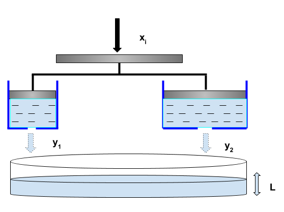
I will attempt to explain this with the help of the visual below. Consider \(x_i\) as the force acting on a horizontal steel plate which is rigidly attached to two pistons inside two cylinders. The volume of water flowing out of each of these cylinders (denoted by \(y_1\) & \(y_2\)) is a function of \(x_i\). The water level \(L\) in the container below is a function of each of \(y_1\) and \(y_2\). Therefore, if I want to find the gradient of \(L\) w.r.t \(x_i\), then I will need to consider the impact of a change in \(x_i\) on each of \(y_1\) and \(y_2\).

With chain rule out of the way, let’s focus on Equation 1. The layer has already receoved Exp. 1 as an input for the backward pass. We need to compute Exp. 2.

\[\begin{align} \frac {\partial y_k}{\partial x_i} &= \frac{\partial y_k}{\partial \hat{x_k}} \times \frac{\partial \hat {x_k}}{\partial x_i} \tag{Exp. 2} \\ \\ &= \frac{\partial (\gamma \hat{x} + \beta)}{\partial \hat {x_k}} \times \frac{\partial \hat {x_k}}{\partial x_i} \\ \\ &= \gamma \frac{\partial \hat {x_k}}{\partial x_i} \\ \\ &= \gamma \frac{\partial \left( {\frac {(x_k - \mu)}{\sqrt{\sigma^2 + \epsilon}}} \right)}{\partial x_i} \\ \\ &= \gamma \left( \frac{\partial \left( {\frac {x_k}{\sqrt{\sigma^2 + \epsilon}}} \right)}{\partial x_i} - \frac{\partial \left( {\frac {\mu}{\sqrt{\sigma^2 + \epsilon}}} \right)}{\partial x_i} \right) \\ \\ &= \gamma \left( \left( \frac{1}{\sqrt{\sigma^2 + \epsilon}} \right) \frac{\partial x_k}{\partial x_i} + x_k \frac{\partial \left({\frac {1}{\sqrt{\sigma^2 + \epsilon}}} \right) }{\partial x_i} - \left( \frac{1}{\sqrt{\sigma^2 + \epsilon}} \right)\frac {\partial \mu}{\partial x_i} - \mu \left( \frac{\partial \left( {\frac {1}{\sqrt{\sigma^2 + \epsilon}}} \right)}{\partial x_i} \right) \right) \\ \\ \end{align}\]

Now we compute some intermediate results:

\[\begin{align} \frac {\partial x_k}{\partial x_i} &= 1(k == i) \tag{2.1} \\ \\ \frac{\partial \sigma^2}{\partial x_i} &= \frac {\partial \left( \frac {1}{N} \sum_{j=1}^N{(x_j - \mu)^2} \right)} {\partial x_i} \tag{2.2} \\ &= \frac{1}{N} \left( \frac{-2}{N}\sum_{j=1, j \ne i}^N{(x_j - \mu)} + 2(x_i - \mu)\left(1 - \frac{1}{N}\right) \right) \\ &= \frac{2}{N}(x_i - \mu) \\ \\ \frac {\partial \left( \frac{1}{\sqrt{\sigma^2 + \epsilon}} \right)}{\partial x_i} &= -\frac{1}{2}(\sigma^2 + \epsilon)^{-\frac{3}{2}} \times \frac{\partial \sigma^2}{\partial x_i} \tag{2.3} \\ &= -\frac{1}{N}(\sigma^2 + \epsilon)^{-\frac{3}{2}} \times (x_i - \mu) \\ \\ \end{align}\]

Substituting the values computed in Equations \(2.1, \space 2.2 \space and \space 2.3\) in \(Exp. \space2\), we get an elegant expression:

\[\begin{align} \frac {\partial y_k}{\partial x_i} &= \frac {\gamma}{\sqrt{\sigma^2 + \epsilon}} \left( {1(k == i) - \frac{1}{N} - \frac{1}{N}\left({\frac{x_i - \mu}{\sqrt{\sigma^2 + \epsilon}}}\right)}\left({\frac{x_k - \mu}{\sqrt{\sigma^2 + \epsilon}}}\right) \right) \tag{2.4} \end{align}\]

Substituting the result in \(2.4\) in our Gradient equation, we get:

\[\begin{align} \frac {\partial L}{\partial x_i} &= {\frac {\gamma}{\sqrt{\sigma^2 + \epsilon}}} \left( \sum_{k=1}^N{\frac{\partial L}{\partial y_k} \times 1(k == i)} - \frac{1}{N}\sum_{k=1}^N{\frac{\partial L}{\partial y_k}} - \frac{1}{N} \sum_{k=1}^N \left({\frac{x_i - \mu}{\sqrt{\sigma^2 + \epsilon}}}\right)\left({\frac{x_k - \mu}{\sqrt{\sigma^2 + \epsilon}}}\right) \right) \\ &= {\frac {\gamma}{\sqrt{\sigma^2 + \epsilon}}} \left( \frac{\partial L}{\partial y_i} - \frac{1}{N}\sum_{k=1}^N{\frac{\partial L}{\partial y_k}} - {\frac{1}{N}\left({\frac{x_i - \mu}{\sqrt{\sigma^2 + \epsilon}}}\right) \sum_{k=1}^N {\frac{\partial L}{\partial y_k}\left({\frac{x_k - \mu}{\sqrt{\sigma^2 + \epsilon}}}\right)} }\right) \\ &= {\frac {\gamma}{\sqrt{\sigma^2 + \epsilon}}} \left( \frac{\partial L}{\partial y_i} - \frac{1}{N}\sum_{k=1}^N{\frac{\partial L}{\partial y_k}} - \frac{1}{N} \hat {x_i} \sum_{k=1}^N {\hat {x_k}\frac{\partial L}{\partial y_k}} \right) \\ \end{align}\]

This can be implemented in Python in a single line: