SVD Part 1 - Introduction to Singular Value Decomposition

In this post I will try to explain what is SVD and what is it good for, with the help of examples. Just as we can write a non-prime number such as 42 as a product of its factors (e.g. as $6\times7$ or as $2\times3\times7$), we can use SVD to write any matrix as a product of three matrices. Why do we need to factorize a matrix? How can we interpret the factors provided by SVD? These are the questions I will attempt to answer. You may check out my Python Notebook which reproduces the illustrations I have used below.

Terminology

Let A be a matrix of size (m,n), i.e. it has m rows and n columns. SVD factorizes A into three matrics:

\[A = U_{m \times r} D_{r \times r} V^T_{r \times n}\]

These factor matrices have some interesting properties, which we will explore below.

P.S. The number r is the Rank of the matrix A. I will not delve into the details, but loosely here’s what it is. Consider a set S of $m \times 1$ vectors which has the property that each column of A can be written as a linear combination of vectors from S. Then the Rank is size of the smallest such set S which exists.

Preliminaries

It is useful to view our mxn matrix A as a collection of m points located in an n-dimensional space (i.e. each row of A represents a point in $\mathbb{R}^{n}$). For example, the matrix below gives us the location of 4 points in 3D space:

\[A = \begin{pmatrix} 1 & 1 & 1 \\ 2 & 3 & 2 \\ 1 & 2 & 3 \\ 4 & 2 & 1 \\ \end{pmatrix}\]

If we use the Cartesian Coordinate System, we can describe each point by three numbers, one for each of the x, y, and z axes. In other words, we can describe the point (1, 2, 3) as a linear combination of three vectors, each of which represents one of x, y, and z axes:

\[\begin{pmatrix} 1 \\ 2 \\ 3 \\ \end{pmatrix} = 1 \times \begin{pmatrix} 1 \\ 0 \\ 0 \\ \end{pmatrix} + 2 \times \begin{pmatrix} 0 \\ 1 \\ 0 \\ \end{pmatrix} + 3 \times \begin{pmatrix} 0 \\ 0 \\ 1 \\ \end{pmatrix}\]

Note that we can represent any point in $\mathbb{R}^3$ as a linear combination of these three vectors - these three vectors are thus said to Span the whole of $\mathbb{R}^{3}$ and are collectively said to form a Basis for $\mathbb{R}^{3}$.

This particular Basis has two properties:

The Basis vectors are pairwise perpendicular.
The length of each Basis vector is 1.

Due to these properties we refer to this Basis as an Orthogonal Basis. Note that this Orthonormal Basis is not unique - multiply one of these Basis vectors by negative one, and the resulting Basis is still Orthonormal.

Punchline: SVD will give us a “Best Fit” Orthonormal Basis for our collection of points. This means that (1) we will be able to represent each of our points as a linear combination of these Basis vectors, and (2) this will be the ‘Best Fit’ Basis among all such Orthonormal Bases.

In what sense is it ‘Best’? If we project our points on each of the Basis vectors given by SVD, the sum of squared lengths of those projections will be the maximum for any such Orthonormal Basis that exists.

Why do we care about this ‘Best Fit’? The intuition is that using vectors from this ‘Best Fit’ Basis, we will be able to a convey a decent amount of information about our matrix, more efficiently than we could convey if we were to use our matrix as it is.

Singular Vectors (The V Matrix)

The ‘Best Fit’ Orthonormal Basis described above is given by the columns of matrix V. Further, there exists a heirarchy among those Basis vectors, with the first column of V, call it V1, being the First Singular Vector - a vector which represents the line through origin which ‘Best Fits’ our collection of points. The second column, V2, being the vector perpendicular to V1, which ‘Best Fits’ our points, and so on.

Let us visualize it with the help of an example in 2D. Consider a collection of two points: (1, 2) and (3, 6). Note that these two points and the origin lie on a straight line. Therefore, the First Singular Vector should simply be a unit vector along the line passing through the origin and these two points! This is indeed what we find out when we perform SVD on a 2x2 matrix containing these points - the blue line in the figure below plots the line given by the First Singular Vector.

Figure 1: Visualization of Orthonormal Basis in 2D

Singular Vectors

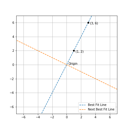
Intuitively, instead of describing our collection of points using two ‘directions’ (which are x and y in the Cartesian system), we have managed to describe the points using a single ‘direction’ (which is along the First Singular Vector)! In plain English, we can describe that direction as one in which the change in y is twice of any change in x.

Putting it in yet another way, by using the First Singular Vector to describe our points in this example, we can convey as much ‘informatioin’ about our points, as we could be describing it in the Cartesian system. Our description is more ‘efficient’ when it comes to the number of ‘directions’ used.

P.S. In the example above, we deliberately chose our points such that one ‘direction’ was enough to explain the entire collection of points. This was just for illustration and one should not expect this to happen in general.

Singular Values (The D Matrix)

Once we have found the kth Singular Vector of our matrix A, its corresponding Singular Value is denoted by $\sigma_{k}$. The number $\sigma_{k}^{2}$ equals the sum of squared projection lengths of each of the points in A (each row of A represents a point) on $V_{k}$. As expected, $\sigma_{1}$ is the largest among all Singular Values. Now let us see how much ‘information’ can be conveyed by utilizing a subset of vectors in the Best Fit Basis given by the matrix V from SVD.

Real World Example - Image Compression

Let’s consider a real world matrix, a grayscale image of size $405 \times 660$, represented by a matrix A which contains 405 rows and 660 columns. In other words, the matrix describes 405 points in a 660-dimensional space. We compute its Singular Vectors using SVD, which gives us a Basis containing 405 vectors.

\[A_{405 \times 660} = U_{405 \times 405} \space D_{405 \times 405} \space V_{405 \times 660}^{T}\]

We pick the first vector of $V$ (call it $V_{1}$) and compute the ‘projection’ of each row of $A$ on $V_{1}$.

Note: The ‘projection’ of a vector $\hat a$ on $\hat b$, a unit vector (i.e. a vector whose length equals 1), is given by $\lt \hat a \cdot \hat b \gt \hat b$ where $\lt \cdot \gt$ denotes the dot product (and it is a scalar quantity).

In our example, each row of A represent a vector of shape $1 \times 660$ (i.e. each row of $A$ represents a point in 660-dimensional space) and we want to compute the ‘projection’ of each such point on $V_{1}$, which is a unit vector of shape $660 \times 1$. Using Pythonic notation, let $A[0,:]$ represent the first row of our image matrix. Then the projection of this row on $V_1$ is given by the vector:

\[\text{Projection of A[0,:] on $V_1$} = \underbrace{<A[0,:], V_1>}_{\text{Length of projection on $V_1$}} \space \underbrace{V_1}_{\text{Unit vector}}\]

Note: This is a good time to introduce some important terminology. We can calculate projection lengths of ALL rows of matrix $A$ on vector $V_1$ through the matrix product $AV_1$. This matrix product is also known as the First Principal Component of $A$.

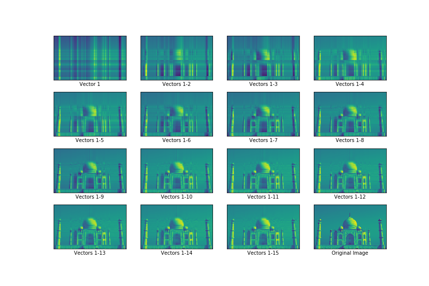
The first image in the figure below shows the projection of $A$ on $V_{1}$ - it doesn’t tell us much about the original image. But as we incrementally utilize more Singular Vectors, we start to form a clearer image. By the time we have utilized the first 15 Singular Vectors (out of a toal of 405 such vectors), our image looks like a decent approximation of the original image (shown as the last image in the figure).

Figure 2: Visualization of First Few Singular Vectors

SVD Results

Quantifying the Efficiency Gain in our Example

If I wanted to share information about the image used in the example above with someone, I have a few choices. I could choose to send the entire original image, in which case I will need to share $267,300 \space (405 \times 660)$ numbers. Instead, if were to share the first 15 Singular Vectors ($9,900 \space (15 \times 660)$ numbers), and the projection lengths of A on each of the $15$ Singular Vectors ($6,075 \space (405 \times 15)$ numbers, I would only need to share a total of $15,975$ numbers, and yet I would manage to convey a decent amount of information. That’s a significant saving!