Introduction

In this post I will derive the key mathematical results used in backpropogation through a Recurrent Neural Network (RNN), popularly known as Backpropogation Through Time (BPTT). Further, I will use the equations I derive to build an RNN in Python from scratch (check out my notebook), without using libraries such as Pytorch or Tensorflow.

Several other resources on the web have tackled the maths behind an RNN, however I have found them lacking in detail on how exactly gradients are “accumulated” during backprop to deal with “tied weights”. Therefore, I will attempt to explain that aspect in a LOT of detail in this post.

I will assume that the reader is familiar with an RNN’s structure and their utility. I highly recommend reading Chapter 10 on ‘Sequence Modelling’ from the book Deep Learning by Goodfellow, Bengio, and Courville.

Each layer of an RNN uses the same copy of parameters (in RNN parlance, weights and biases are “tied together”) - this is unlike a plain feedforward network where each layer has its own set of parameters. This aspect makes understanding backpropogation through an RNN a bit tricky.

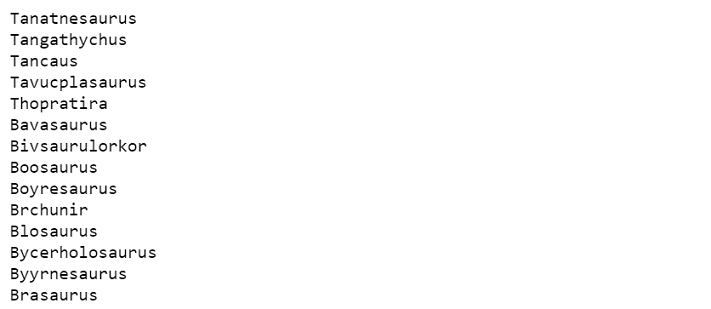
I will also use the RNN model I build, to train a simple character-level model on a dataset of real dinosaur names. This model throws out some interesting names (see below) such as ‘Boosaurus’!

Figure: Sample Dinosaur Names Generated by my RNN Model

Terminology

To process a sequence of length \(T\), an RNN uses \(T\) copies of a Basic Unit (henceforth referred to as just a Unit). In the figure below, I have shown two Units of an RNN. The parameters used by each Unit are “tied together”. That is, the weight matrices \(W_h\), \(W_e\) and biases \(b_1\) and \(b_2\), are the same for each Unit. Each Unit is also referred to as a “time step”.

Figure: Structure of a Recurrent Neural Network (showing two ‘time-steps’)

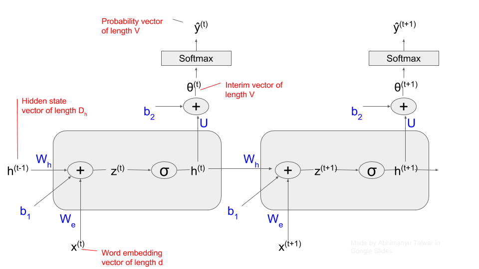
The parameters used by this RNN are the weight matrices \(W_h\), \(W_e\), and \(U\), and the bias vectors \(b_1\) and \(b_2\). During backprop, we need to calculated gradients of the training loss with respect to all of these parameters.

Notation

Throughout this blog post:

• Superscript \((t)\), such as in \(h^{(t)}\) refers to value of a variable (in this case \(h\)) at time-step \(t\).
• Subscript \([i]\) in square brackets, such as in \(h^{(t)}_{[i]}\) refers to the \(i^{th}\) component of the vector \(h^{(t)}\).
• The symbols \(\times\) and \(\circ\) refer to scalar and element-wise multiplication respectively. In absence of a symbol, assume matrix multiplication.
• Superscript \(Tr\), such as in \(W_h^{Tr}\), implies Transpose of the matrix \(W_h\).

An entire RNN can be broken down into three parts - I discuss each of those below. I recommend referring to the diagram of an RNN’s structure above while reading about the three parts below:

(1) RNN Unit Computation

The RNN Unit at time-step \(t\) takes as inputs:

• \(x^{(t)}\), a vector of dimensions \(d \times 1\), which represents the \(t^{th}\) ‘word’ in a sequence of length \(T\), and
• \(h^{(t-1)}\), a vector of dimensions \(D_h \times 1\), which is the output of the previous RNN Unit, and is referred to as a ‘hidden-state’ vector.

Note: The numbers \(D_h\) and \(d\), which represent the lengths of the ‘hidden-state’ and the input embedding vectors, respectively, are ‘hyperparamters’. That is, it is up to us to choose values for these numbers.

The output of the RNN unit at time-step \(t\) is its ‘hidden-state vector’ \(h^{(t)}\). The equations governing a single unit are: \(\begin{align} z^{(t)} &= W_h h^{(t-1)} + W_x x^{(t)} + b_1 \tag{1.1} \\ h^{(t)} &= \sigma(z^{(t)}) \tag{1.2} \end{align}\)

Note: \(W_h\) is a square matrix of dimensions \(D_h \times D_h\). The matrix \(W_x\) has dimensions \(D_h \times d\).

The symbol \(\sigma()\) refers to the Sigmoid function, defined as:

\[\sigma(x) = \frac{1}{(1 + e^{-x})}\]

The derivative of \(\sigma(x)\) (with respect to x) is straightforward to compute:

\[\sigma'(x) = \sigma(x) \times (1 - \sigma(x))\]

An RNN comprises a sequence of a number of such single RNN Units. It is evident from these equations that a perturbation to the weight matrix \(W_h\) will impact the value of a hidden-state vector \(h^{(t)}\) not just directly via its presence in \(Eq. 1.1\), but also indirectly via its impact on all hidden-state vectors \(h^{(1:t-1)}\). This aspect of an RNN makes the gradient calculations seem tricky but we will see two clever work-arounds to tackle this.

(2) The Affine Layer

The hidden-state vector \(h^{(t)}\) of RNN Unit at time-step \(t\) is fed into (1) the next RNN Unit, and (2) through an Affine Layer which produces the vector \(\theta^{(t)}\) of dimensions \(V \times 1\), where \(V\) is the size of our Vocabulary (set of all ‘words’ in our training-set if you are passing a word vector as input \(x^{(t)}\) at time-step \(t\), or a set of all characters in our training set if we are working on a character level RNN Model). The equations governing this layer are:

\[\theta^{(t)} = Uh^{(t)} + b_2 \tag{2.1}\]

(3) The Softmax Layer

This layer uses the \(\theta^{(t)}\) vector generated by the Affine Layer for time-step \(t\) and computes a probability distribution for the next word for this time step. The distribution is a vector \(\hat{y}^{(t)}\) of dimensions \(V \times 1\). The probability that the next word is at index \(i\) in the Vocabulary is given by:

\[\hat{y}^{(t)}_{[i]} = \frac {e^{\theta^{(t)}_{[i]}}} {\sum_{j=0}^{V-1} e^{\theta^{(t)}_{[i]}}} \tag{3.1}\]

And finally the loss attributed to this time-step, \(J^{(t)}\) is given by:

\[J^{(t)} = -\sum_{i=0}^{V-1} y^{(t)}_{[i]} log \hat{y}^{(t)}_{[i]} \tag{3.2}\]

The vector \(y^{(t)}\) is a one-hot vector with the same dimensions as that of \(\hat{y}^{t}\) - it contains a \(1\) at the index of the ‘true’ next-word for time-step \(t\). And finally, the overall loss for our RNN is the sum of losses contributed by each time-step:

\[J = \sum_{t=1}^{T} J^{(t)} \tag{3.3}\]

GOAL: We want to find the gradient of \(J\) with respect to each and every element of parameter matrices and vectors \(W_h\), \(W_x\), \(b_1\), \(U\), and \(b_2\). For the sake of length of this post, I will only demonstrate all the maths required to calculate gradients w.r.t \(W_h\), but I believe that after reading this, you will be able to apply the same concepts for other parameters.

The First BPTT Trick: Dummy Variables

Parameters such as \(W_h\) influence the loss for a single time-step \(J^{(t)}\), not just through their direct role in computation of the hidden-state \(h^{(t)}\) (see \(Eq. 1.1\) and \(Eq. 1.2\)) but also via their influence on all the previous hidden-states \(h^{(0:t-1)}\). So if we use the chain-rule to write the partial derivative of \(J^{(t)}\) with respect to \(W_h\), we will end up with a complex expression which includes contributions from each time-step from time-step \(0\) to \(t\).

That can be simplified (I’ll explain this below) if we pretend that the \(W_h\) used at each time step is a dummy variable, \(W_h^{(t)}\), with each such dummy variable mapped to the original weight matrix \(W_h\) by the simple identity mapping (that’s basically just saying \(W_h^{(t)} = W_h\)).

Using dummy variables allows us to break the gradient of loss \(J^{(t)}\) with respect to the \([i, j]^{th}\) element of \(W_h\), into a simpler sum of parts.

\[\begin{align} \frac {\partial J^{(t)}} {\partial W_{h [i,j]}} &= \sum_{k=1}^{T} \frac {\partial J^{(t)}} {\partial W_{h [i,j]}^{(k)}} \times \underbrace{\frac {\partial W_{h [i,j]}^{(k)}} {\partial W_{h[i,j]}}}_{Equals \space 1.} \\ \\ &= \sum_{k=1}^{T} \frac {\partial J^{(t)}} {\partial W_{h [i,j]}^{(k)}} \tag{4.1}\\ \end{align}\]

How does this simplify our job? To compute gradient of \(J^{(t)}\) with respect to \(W_h\) in a single expression, we will need to factor in contributions from all time-steps. But if our task now is computing gradients w.r.t \(W_h^{(k)}\), we only need to look at contributions from time-steps \([k, k+1, \cdots, t-1, t]\) (because \(W_h^{(k)}\) does not influence any variables computed prior to time-step \(k\)). In the spirit of backprop, we now rely only on values computed ‘ahead’ of us in the computational graph.

Blueprint for Computing RNN Gradients

Before delving into calculus, two big picture questions are:

• What information do we need at each time-step to compute gradients?
• How do we pass that information efficiently between layers?

Let’s start by answering these two questions for gradients of loss from the \(t^{th}\) step, \(J^{(t)}\) w.r.t. \(W_{h[i,j]}^{(k)}\). I’ll make (and prove!) two claims below which will help us out.

Claim 1: At any given time-step \(k\), if we know the value of \(\frac {\partial J^{(t)}} {\partial h^{(k)}}\) (denoted by \(\gamma_t^{(k)}\) from here on), we can compute gradients w.r.t. the weight matrix \(\underline{for \space the \space k^{th} \space step}\), i.e. \(\frac {\partial J^{(t)}} {\partial W_{h}^{(k)} }\).

Proof: Using the chain rule:

\[\begin{align} \frac {\partial J^{(t)}} {\partial W_{h[i,j]}^{(k)}} &= \sum_{p=1}^{D_h} \underbrace{\frac {\partial J^{(t)}} {\partial h_{[p]}^{(k)}}}_{\gamma_{t[p]}^{(k)}} \times \underbrace{\frac {\partial h_{[p]}^{(k)}} {\partial W_{h[i,j]}^{(k)}} }_{\text{See Eq. 5.1}} \tag{5.0} \\ \end{align}\]

As we have assumed we know \(\gamma_t^{(k)}\), the first quantity on the right hand side is taken care of. If we can show that at time-step \(k\), we have adequate information to compute the second quantity, then we’ve proved this claim.

Using the chain rule and the relationship between the hidden-state \(h^{(k)}\) and interim variable \(z^{(k)}\) from \(Eq. \space 1.2\):

\[\begin{align} \frac {\partial h_{[p]}^{(k)}} {\partial W_{h[i,j]}^{(k)}} &= \sum_{m=1}^{D_h} \underbrace{\frac {\partial h_{[p]}^{(k)}} {\partial z_{[m]}^{(k)}}}_{\text{Eq. 5.1.1}} \times \underbrace{\frac {\partial z_{[m]}^{(k)}} {\partial W_{h[i,j]}^{(k)}}}_{\text{Eq. 5.1.2}} \tag{5.1} \end{align}\]

Evaluating the two quantities on the right hand side:

\[\begin{align} \frac {\partial h_{[p]}^{(k)}} {\partial z_{[m]}^{(k)}} &= \begin{cases} 0, & \text{p $\ne$ m} \\[2ex] \sigma' (z_{[p]}^{(k)}), & \text{p = m} \tag{5.1.1} \end{cases} \end{align}\] \[\begin{align} \frac {\partial z_{[m]}^{(k)}} {\partial W_{h[i,j]}^{(k)}} &= \begin{cases} 0, & \text{m $\ne$ i} \\[2ex] h_{[j]}^{(k-1)}, & \text{m = i} \tag{5.1.2} \end{cases} \end{align}\]

Substituting in \(Eq. 5.1\) we get,

\[\begin{align} \frac {\partial h_{[p]}^{(k)}} {\partial W_{h[i,j]}^{(k)}} &= \begin{cases} 0, & \text{p $\ne$ i} \\[2ex] \sigma' (z_{[i]}^{(k)}) \times h_{[j]}^{(k-1)}, & \text{p = i} \end{cases} \end{align}\]

Substituting this result in \(Eq. 5.0\) we get,

\[\begin{align} \frac {\partial J^{(t)}} {\partial W_{h[i,j]}^{(k)}} &= \gamma_{t[i]}^k \times \sigma' (z_{[i]}^{(k)}) \times h_{[j]}^{(k-1)} \end{align}\]

Voila! We have all the information required to compute the expression above at time-step \(k\) (each of the vectors \(z^{(k)}\) and \(h^{(k-1)}\) can be cached during a forward pass). In matrix terms, we can now write the gradient as:

Writing the final result in matrix terms (with \(\circ\) denoting elementwise multiplication of vectors),

\[\bbox[yellow,5px,border:2px solid red] { \frac {\partial J^{(t)}} {\partial W_{h}^{(k)}} = (\underbrace{\gamma_{t}^{(k)}}_{\text{???}} \circ \underbrace{\sigma' (z^{(k)})}_{\text{Local}}) \times (\underbrace{h^{(k-1)}}_{\text{Local}})^{Tr} \qquad (5.2) }\]

Two out of three quantities required to compute this gradient are available locally (they were cached during our forward-pass for time-step \(k\)). But how do we get \(\gamma_{t}^{(k)}\)? Moreover, here we’ve just computed the gradient of \(J^{(t)}\) w.r.t \(W_h^{(k)}\) - in order to complete our backprop, we will need gradient of each of \(J^{(k)}, \cdots, J^{(t)}, \cdots, J^{(T)}\) w.r.t. to \(W_h^{(k)}\). Looks like we will need a lot of values of \(\gamma\) to compute the full gradient for loss w.r.t \(W_h^{(k)}\).

How do we pass all this information to time-step \(k\)? This is where our second Claim wil rescue us. To state the problem we have at hand clearly, at time-step \(k\), we need values of each of \(\gamma_{k}^{(k)}, \gamma_{k+1}^{(k)}, \cdots, \gamma_{T-1}^{(k)}, \gamma_{T}^{(k)}\) to compute full-gradient of loss of the RNN w.r.t \(W_h^{(k)}\)

Claim 2: At time-step \(k\), given \(\gamma_{t}^{(k)}\), we can compute \(\gamma_{t}^{(k-1)}\) using only locally available information (i.e. information which was cached during the forward-pass through time-step \(k\)).

Proof: Using chain rule:

\[\begin{align} \gamma_{t[j]}^{(k-1)} &= \frac {\partial J^{(t)}} {\partial h_{[j]}^{(k-1)}} \\ &= \sum_{i=1}^{D_h} \underbrace{\frac {\partial J^{(t)}} {\partial h_{[i]}^{(k)}}}_{\gamma_{t[i]}^{(k)}} \times \underbrace{\frac {\partial h_{[i]}^{(k)}} {\partial h_{[j]}^{(k-1)}}}_{\text{Eq. 6.1}} \tag{6.0} \end{align}\]

Let’s calculate the second quantity on the right hand side. Using the chain rule:

\[\begin{align} \frac {\partial h_{[i]}^{(k)}} {\partial h_{[j]}^{(k-1)}} &= \sum_{p=1}^{D_h} \underbrace{\frac {\partial h_{[i]}^{(k)}} {\partial z_{[p]}^{(k)}}}_{\text{Eq. 6.1.1}} \times \underbrace{\frac {\partial z_{[p]}^{(k)}} {\partial h_{[j]}^{(k-1)}}}_{\text{Eq. 6.1.2}} \tag{6.1} \end{align}\]

So we have this straightforward Sigmoid derivative:

\[\begin{align} \frac {\partial h_{[i]}^{(k)}} {\partial z_{[p]}^{(k)}} &= \begin{cases} 0, & \text{i $\ne$ p} \\[2ex] \sigma'(z_{[i]}^{(k)}), & \text{i = p} \tag{6.1.1} \end{cases} \end{align}\]

And using \(Eq. 1.1\), we have:

\[\begin{align} \frac {\partial z_{[p]}^{(k)}} {\partial h_{[j]}^{(k-1)}} &= W_{h[p,j]}^{(k)} \tag{6.1.2} \\ \end{align}\]

Using \(Eq. 6.1.1\) and \(Eq. 6.1.2\) in \(Eq. 6.1\), we get:

\[\begin{align} \frac {\partial h_{[i]}^{(k)}} {\partial h_{[j]}^{(k-1)}} &= \sigma'(z_{[i]}^{(k)}) \times W_{h[i,j]}^{(k)} \end{align}\]

Now using these results in \(Eq. 6.0\), we get:

\[\begin{align} \gamma_{t[j]}^{(k-1)} &= \sum_{i=1}^{D_h} \gamma_{t[i]}^{(k)} \times \sigma'(z_{[i]}^{(k)}) \times W_{h[i,j]}^{(k)}) \end{align}\]

In matrix terms:

\[\bbox[yellow,5px,border:2px solid red] { \gamma_{t}^{(k-1)} = (W_{h}^{(k)})^{Tr} (\gamma_{t}^{(k)} \circ \sigma'(z_{}^{(k)})) \qquad (6.2) }\]

Note: Just a reminder for notation - \(A^{Tr}\) stands for Transpose of the matrix \(A\).

This proves Claim 2! Phew! Let us take a moment to understand why this equation, \(Eq. 6.2\), is useful for our task.

Given \(\gamma_{t}^{(k)}\) at time-step \(k\), we have already proved in Claim 1 (see \(Eq. 5.2\)) that we can compute gradient of \(J^{(t)}\) w.r.t \(W_h^{(k)}\). In Claim 2, we have now proved that using \(\gamma_{t}^{(k)}\), we can also compute \(\gamma_{t}^{(k-1)}\), which can be used by time-step \((k-1)\) to compute gradient of \(J^{(t)}\) w.r.t \(W_h^{(k-1)}\).

Now if we start at time-step \(t\) with \(\gamma_{t}^{(t)}\) (which is straightforward to calculate - just backprop through the Softmax and Affine Layers), we can successively calculate \(\gamma_{t}^{(t-1)}, \space \gamma_{t}^{(t-2)}, \cdots, \gamma_{t}^{(2)}, \space \gamma_{t}^{(1)}\) through applications of \(Eq. 6.2\), and at each step, compute gradients of \(J^{(t)}\) w.r.t \(W_h^{(t-1)}, \space W_h^{(t-2)}, \cdots, W_h^{(2)}, \space W_h^{(1)}\) through applications of \(Eq. 5.2\).

We have now managed to computie gradient of \(J^{(t)}\) w.r.t \(W_h^{(k)}\) for all \(k \in [1, \cdots, t]\)! But we are not done yet! We need to do this for all values of \(t \in [0, \cdots, T]\). Does that mean we need to run backprop (which involves a pass through \(T\) RNN units), \(T\) times? As we will see, that is not required, and a single backprop run will be enough.

The Second BPTT Trick: Accumulating Gradients

Following the train of thought above, to compute gradient of \(J^{(t)}\) w.r.t \(W_h^{(k)}\) for all values of \(t \in [k, \cdots, T]\), the time-step k should receive \(\gamma_{t}^{(k)}\) for all values of \(t \in [k, \cdots, T]\) so that we can apply \(Eq. 5.2\) to compute the required gradients. And the table below shows how time-step \(k\) can receive this information!

\[\begin{array}{c|ccc|ccc|ccc} \text{Time Step} & \text{Compute} & \text{Current} & \text{Time Step} & \text{To} & \text{Previous} & \text{Time Step} & \text{Gradients} & & \text{Accumulated}\\ \hline T & \gamma_T^{(T)} & & & \gamma_T^{(T-1)} & & & \frac {\partial J^{(T)}} {\partial W_h^{(T)}} & & \\[2ex] T-1 & \gamma_{T-1}^{(T-1)} & \gamma_{T}^{(T-1)} & & \gamma_{T-1}^{(T-2)} & \gamma_{T}^{(T-2)} & & \frac {\partial J^{(T-1)}} {\partial W_h^{(T-1)}} & \frac {\partial J^{(T)}} {\partial W_h^{(T-1)}} & \\[2ex] T-2 & \gamma_{T-2}^{(T-2)} & \gamma_{T-1}^{(T-2)} & \gamma_{T}^{(T-2)} & \gamma_{T-2}^{(T-3)} & \gamma_{T-1}^{(T-3)} & \gamma_{T}^{(T-3)} & \frac {\partial J^{(T-2)}} {\partial W_h^{(T-2)}} & \frac {\partial J^{(T-1)}} {\partial W_h^{(T-2)}} & \frac {\partial J^{(T)}} {\partial W_h^{(T-2)}} \\ \end{array}\]

For each time-step \(k\), the columne titled Compute Current Time Step lists quantities which can either be computed locally (such as \(\gamma_k^{(k)}\)) or those which are received from time-step \((k+1)\) during backpropogation. The first observation is that at each time-step \(k\), this columns lists quantities which will through \(Eq. 5.2\), allow us to compute gradients of \(J^{(t)}\) w.r.t \(W_h^{(k)}\) for all \(t \in [k, \space k+1, \cdots, T-1, \space T]\). Go back to \(Eq. 5.2\) to convince yourself!

The last column, titled Gradients Accumulated, shows the gradients which are calculated at this time-step through application of \(Eq. 5.2\) on values in the \(2^{nd}\) column.

The column titled To previous Time Step lists quantities which are passed on from this time-step to its previous time-step during backpropogation. For instance, at time-step \(T\), we compute \(\gamma_T^{(T)}\) (by a simple backprop of \(J^{(T)}\) through Softmax and Affine layers), and then use it to compute \(\gamma_T^{(T-1)}\) by employing \(Eq. 6.2\) which we had derived above. We pass this quantity on to time-step \(T-1\).

Now it gets interesting - at time-step \(T-1\), we’ve got the locally computed \(\gamma_{T-1}^{(T-1)}\) and we’ve also received \(\gamma_T^{(T-1)}\) from time-step \(T\). We can again apply \(Eq. 6.2\) on these two quantities to compute the \(3^{rd}\) column of our table. But now we have two values which we want to pass on to time-step \((T-2)\)!! How do we do that?

It turns out that we can sum them up and pass that sum (instead of two individual values) on to time-step \(T-2\). At time-step \((T-2)\), consider the application of \(Eq. 6.2\) to the sum of \(\gamma_{T-1}^{(T-2)}\) and \(\gamma_{T}^{(T-2)}\) received from time-step \(T-1\):

\[\begin{align} (W_{h}^{(k)})^{Tr} (\left[ \gamma_{T-1}^{(T-2)} + \gamma_{T}^{(T-2)} \right] \circ \sigma'(z_{}^{(k)})) \end{align}\]

Now both element-wise multiplication and matrix multiplication are Distributive, i.e. given vectors \(a\), \(b\), and \(c\):

\[a \circ (b + c) = (a \circ b) + (a \circ c)\]

And given matrices \(A\), \(B\), and \(C\):

\[A(B + C) = AB + AC\]

Therefore we have:

\[\begin{align} (W_{h}^{(k)})^{Tr} (\left[ \gamma_{T-1}^{(T-2)} + \gamma_{T}^{(T-2)} \right] \circ \sigma'(z_{}^{(k)})) &= (W_{h}^{(k)})^{Tr} (\gamma_{T-1}^{(T-2)} \circ \sigma'(z_{}^{(k)})) + (W_{h}^{(k)})^{Tr} (\gamma_{T}^{(T-2)} \circ \sigma'(z_{}^{(k)})) \\ &= \gamma_{T-1}^{(T-3)} + \gamma_{T}^{(T-3)} \end{align}\]

There we go! By passing on the sum of quantities we wanted to pass to time-step \((T-2)\) from \((T-2)\), we’ve managed to get the sum of the quantities we needed in the \(3^{rd}\) column at time-step \((T-2)\). But you may ask whether computing the sum of quantities required at time-step \((T-2)\), is as good as computing individual quantities? The answer is YES!

In order to compute gradients, we will apply \(Eq. 5.2\) - and the expression for \(Eq. 5.2\) tells us that all operations in it are also Distributive! So the application of \(Eq. 5.2\) to sum of gammas will give us the sum of the gradients we want. This efficient method of backpropogating by passing sums is referred to as “accumulating gradients”. While this doesn’t allow us to compute \(\frac {\partial J^{(t)}} {\partial W_h^{(k)}}\) individually for values of \(t\) and \(k\), that doesn’t matter - because what ultimately matters is gradient of the total loss \(\frac {\partial J} {\partial W_h}\). And we are able to compute that by accumulating gradients in this manner.

Conclusion

This turned into a longer blog post than I had initially imagined. While I’ve only shown computation of gradients w.r.t. one parameter matrix \(W_h\), I hope this post clarifies the bigger picture concepts of “dummy variables” and “accumulation of gradients”. Using these, you should be able to compute gradients w.r.t other parameters of an RNN as well. If you’re stuck, you may check out the accompanying Python notebook to understand the calculations behind other gradients.

If you find any errors in this post, or have any feedback, I request you to reach out to me on LinkedIn.