TL;DR

In this blog post:

1. I derive equations for Backpropogation-Through-Time (BPTT) for an LSTM.
2. I illustrate proper application of chain-rule: (1) traversing all paths of ‘influence flow’, & (2) avoiding double-counting of paths.
3. I create an LSTM model in Python (using just Numpy/Random libraries): click here to view the Notebook.

Introduction

In my last post on Recurrent Neural Networks (RNNs), I derived equations for backpropogation-through-time (BPTT), and used those equations to implement an RNN in Python (without using PyTorch or Tensorflow). Through that post I demonstrated two tricks which make backprop through a network with ‘tied up weights’ easier to comprehend - use of ‘dummy variables’ and ‘accumulation of gradients’. In this post I intend to look at another neural network architecture known as an LSTM (Long Short-Term Memory), which builds upon RNNs, and overcomes the issue of vanishing gradients faced by RNNs.

The mathematics used is not dissimilar from what is required for RNNs. That said, one has to be careful about the ‘flow of influence’ from various nodes in the network to the network’s loss.

‘Flow of Influence’: Viewing a Neural Network as a Directed Acyclic Graph, if there exists a path from Node A to Node B, then a change in value of A will likely have an impact on B’s value. In other words, ‘influence can flow’ from A to B along the path between them. While applying chain-rule, one should be careful enough to: (1) not exclude any paths of ‘influence flow’ from computation, and (2) not double-count the ‘influence flow’ between two nodes.

I will assume that the reader is familiar with LSTMs. I believe this lecture by Stanford’s Prof. Christopher Manning offers the best explanation of how LSTMs overcome the limitation of ‘vanishing gradients’ observed in RNNs.

I strongly suggest you read my post on RNNs before proceeding because it introduces some key tricks which I will reuse in this post. Also, I will frequently draw parallels (and highlight differences) between the results I proved for RNNs and the ones I prove here.

Terminology

To process a sequence of length \(T\), an LSTM uses \(T\) copies of a Basic Unit (henceforth referred to as just a Unit). Each Unit uses the same set of parameters (weights and biases). One way to understand this is that there is a ‘root’ version of a weight matrix \(W\), and each Unit uses this same version. Any changes to the ‘root’ are reflected in the matrix \(W\) used by each Unit. We sometimes say that the parameters are ‘tied together’ across Units.

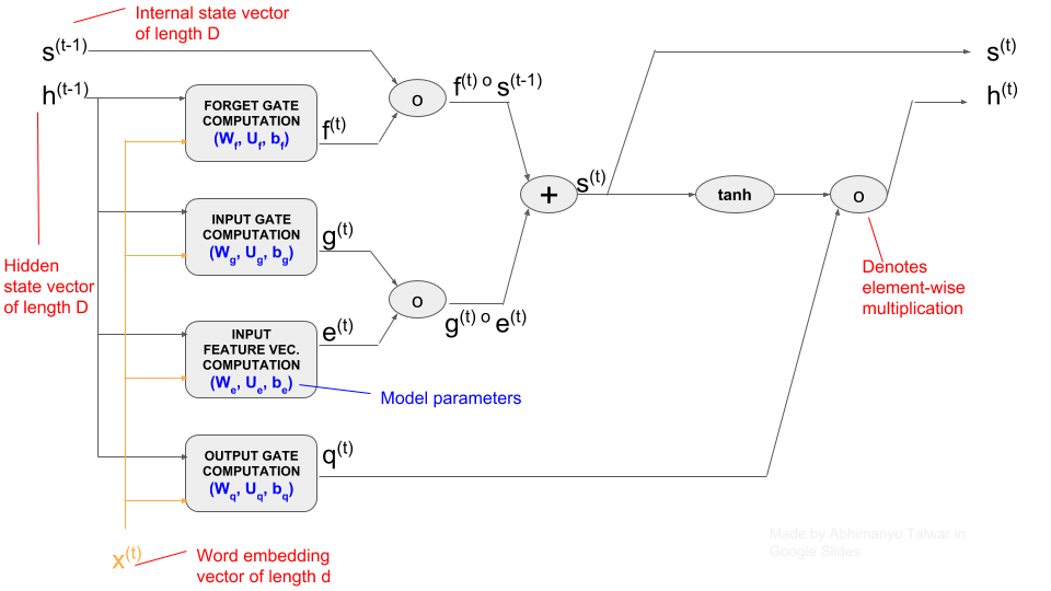
Figure: Structure of an LSTM Network (showing a single LSTM Unit)

Note:

• Variables in blue color are the parameters of the network. We need to learn these parameters through training on data.
• Scroll below for equations that govern the computation inside each of the four rectangular boxes in the diagram.

Notation

I have tried to use the same alphabets to denote various parameters as used in Chapter 10 (Sequence Modelling) of the Deep Learning book by Goodfellow, Bengio, and Courville. I will use the same notation as I used for my blog post on RNNs:

• Superscript \((t)\), such as in \(h^{(t)}\) refers to value of a variable (in this case \(h\)) at time-step \(t\).
• Subscript \([i]\) in square brackets, such as in \(h^{(t)}_{[i]}\) refers to the \(i^{th}\) component of the vector \(h^{(t)}\).
• The symbols \(\times\) and \(\circ\) refer to scalar and element-wise multiplication respectively. In absence of a symbol, assume matrix multiplication.
• Superscript \(Tr\), such as in \(W_f^{Tr}\), implies Transpose of the matrix \(W_f\).

Similar to the case of RNNs, I will break down the computation inside an LSTM into three parts: (1) LSTM Units, (2) Affine Layer, and (3) Softmax Layer. I will cover the computation for LSTM Units in detail in this post. For the sake of completeness, I describe the other two parts briefly below (you may refer to my previous post on RNNs for details).

Affine Layer

This layer applies an Affine Transformation to the ‘hidden-state’ \(h^{(t)}\) at each time-step \(t\), to produce a vector \(\theta^{(t)}\) of length \(V\) (the size of our Vocabulary). The formula below describes the computation (\(U\) and \(b\) are model parameters):

\[\theta^{(t)} = Uh^{(t)} + b \tag{3.0}\]

Softmax Layer:

At each time-step, the vector \(\theta^{(t)}\) is used to compute a probability distribution over our Vocabulary of \(V\) words. The formula below describes this:

\[\hat{y}^{(t)}_{[i]} = \frac {e^{\theta^{(t)}_{[i]}}} {\sum_{j=0}^{V-1} e^{\theta^{(t)}_{[i]}}} \tag{4.0}\]

I have discussed the Affine and Softmax computations in my blog post on RNNs. The same discussion holds for LSTMs as well and so I will not be talking about those layers here.

The loss attributed to this time-step, \(J^{(t)}\) is given by:

\[J^{(t)} = -\sum_{i=0}^{V-1} y^{(t)}_{[i]} log \hat{y}^{(t)}_{[i]} \tag{5.0}\]

The vector \(y^{(t)}\) is a one-hot vector with the same dimensions as that of \(\hat{y}^{t}\) - it contains a \(1\) at the index of the ‘true’ next-word for time-step \(t\). And finally, the overall loss for our LSTM is the sum of losses contributed by each time-step:

\[J = \sum_{t=1}^{T} J^{(t)} \tag{5.1}\]

GOAL: We want to find the gradient of \(J\) with respect to each and every element of parameter matrices and vectors. For the sake of length of this post, I will only demonstrate all the maths required to calculate gradients w.r.t \(W_f\), but I believe that after reading this, you will be able to apply the same concepts for other parameters. You can always refer to my Jupyter Notebook to understand how rest of the gradients should be calculated.

LSTM Unit Computation

The LSTM Unit at time-step \(k\) takes as inputs:

• \(x^{(k)}\), a vector of dimensions \(d \times 1\), which represents the \(t^{th}\) ‘word’ in a sequence of length \(T\), and
• \(h^{(k-1)}\), a vector of dimensions \(D \times 1\), which is the output of the previous LSTM Unit, and is referred to as a ‘hidden-state’ vector.
• \(s^{(k-1)}\), a vector of dimensions \(D \times 1\), which is the output of the previous LSTM Unit, and is referred to as an ‘internal-state’ vector.

Note: The numbers \(D\) and \(d\) are hyperparameters.

LSTM Gates: A distinguishing feature of LSTMs (relative to RNNs) is the presence of three ‘Gates’ in each LSTM Unit. These Gates dampen the values of certain signals coming into and going out of the Unit, through multiplication by some factor which lies between \([0, \space 1]\). There are three Gates: (1) INPUT, denoted by \(g^{(k)}\), which dampens \(x^{(k)}\), (2) FORGET (\(f^{(k)}\)), which dampens \(s^{(k-1)}\), and (3) OUTPUT (\(q^{(k)}\)), which dampens \(h^{(k)}\). Equations \(2.1, 2.2, 2.3\) below specify the exact maths behind these Gates.

Let’s start by looking at how the hidden-state \(h\) and internal-state \(s\) are computed at time-step \(t\):

\[\underbrace{h^{(t)}}_{\substack{\text{hidden} \\ \text{state}}} = \underbrace{q^{(t)}}_{\substack{\text{output} \\ \text{gate}}} \circ tanh(\underbrace{s^{(t)}}_{\substack{\text{internal} \\ \text{state}}}) \tag{1.1}\] \[s^{(t)} = \underbrace{f^{(t)}}_{\substack{\text{forget} \\ \text{gate}}} \circ s^{(t-1)} + \underbrace{g^{(t)}}_{\substack{\text{input} \\ \text{gate}}} \circ \underbrace{e^{(t)}}_{\substack{\text{input} \\ \text{feature} \\ \text{vector}}} \tag{1.2}\]

Now let’s look at how the input feature vector \(e^{(t)}\) and the three gates are computed:

\[\begin{align} \text{(Forget Gate) } f^{(t)} &= \sigma \underbrace{\left( b_{f} + U_{f}x^{(t)} + W_{f}h^{(t-1)} \right)}_{z_f} \tag{2.1} \\ \text{(Input Gate) } g^{(t)} &= \sigma \underbrace{\left( b_{g} + U_{g}x^{(t)} + W_{g}h^{(t-1)} \right)}_{z_g} \tag{2.2} \\ \text{(Output Gate) } q^{(t)} &= \sigma \underbrace{\left( b_{q} + U_{q}x^{(t)} + W_{q}h^{(t-1)} \right)}_{z_q} \tag{2.3} \\ \text{(Input Feature Vector) } e^{(t)} &= \sigma \underbrace{\left( b_{e} + U_{e}x^{(t)} + W_{e}h^{(t-1)} \right)}_{z_e} \tag{2.4} \end{align}\]

The \(tanh\) function, also known as the Hyperbolic Tangent, is defined as follows:

\[tanh(x) = \frac {1 \space - \space e^{-2x}} {1 \space + \space e^{-2x}}\]

Its derivative with respect to \(x\) at a point, can be computed in terms of the value of \(tanh\) at that point:

\[tanh'(x) = (1 \space - \space tanh^{2}(x))\]

Applying the Two BPTT Tricks

We will make use of the two Backpropogation-Through-Time (BPTT) tricks that I had described in detail in my blog post on RNNs. Using the ‘Dummy Variables’ trick, we will pretend that the LSTM Unit at time-step \(k\) has its own copy of parameters. For example instead of the matrices \(W_f\) and \(U_f\), we will pretend that this Unit uses parameters \(W_f^{(k)}\) and \(U_f^{(k)}\). We can say:

\[\begin{align} \frac {\partial J^{(t)}} {\partial W_{f [i,j]}} &= \sum_{k=1}^{T} \frac {\partial J^{(t)}} {\partial W_{f [i,j]}^{(k)}} \times \underbrace{\frac {\partial W_{f [i,j]}^{(k)}} {\partial W_{f[i,j]}}}_{Equals \space 1.} \\ \\ &= \sum_{k=1}^{T} \frac {\partial J^{(t)}} {\partial W_{f [i,j]}^{(k)}} \tag{6.0}\\ \end{align}\]

Blueprint for Computing Gradients

We ask ourselves the same big picture questions which we had asked for RNNs:

1. What information do we need at each time-step to compute gradients?
2. How do we pass that information efficiently between layers? We will find answers to these below.

Tracing Paths of Influence

Observe that our parameter of interest, \(W_f\) appears only in one of the equations, \(Eq. 2.1\). Focussing on the version of \(W_f\) used by the Unit at time-step \(k\), i.e. \(W_f^{(k)}\), we can see that a change in the value of \(W_f^{(k)}\) will cause a change in the value of \(f^{(k)}\), which in turn will impact the value of loss for our LSTM.

We are basically tracing paths through which ‘influence’ could flow from our variable of interest to the value of loss for our LSTM! In this case, we’ve discovered that there is a path from \(W_f^{(k)}\) to the loss quantity \(J^{(t)}\), via \(f^{(k)}\). Moreover, we have observed that there is NO PATH between \(W_f^{(k)}\) and \(J^{(t)}\) which avoids \(f^{(k)}\). Therefore, if we know the gradient of loss w.r.t. \(f^{(k)}\), we can just restrict our task to understanding how ‘influence’ flows from \(W_f^{(k)}\) to \(f^{(k)}\), and we should be able to compute the gradient of loss w.r.t. \(W_f^{(k)}\).

Claim 1: At any given time-step \(k\), if we know the value of \(\frac {\partial J^{(t)}} {\partial s^{(k)}}\) (denoted by \(\delta_t^{(k)}\) from here on), we can compute gradients w.r.t. the weight matrix \(W_f\) \(\underline{for \space the \space k^{th} \space step}\), i.e. \(\frac {\partial J^{(t)}} {\partial W_{f}^{(k)} }\).

Proof: Utilizing our knowledge of the paths of influence from \(W_f^{(k)}\) to \(J^{(t)}\), and using chain-rule, we have:

\[\begin{align} \frac {\partial J^{(t)}} {\partial W_{f[i,j]}^{(k)}} &= \sum_{p=1}^{D} \underbrace{\frac {\partial J^{(t)}} {\partial f_{[p]}^{(k)}}}_{\text{Eq. 6.1.1}} \times \underbrace{\frac {\partial f_{[p]}^{(k)}} {\partial W_{f[i,j]}^{(k)}} }_{\text{Eq. 6.1.2}} \tag{6.1} \\ \end{align}\]

The second quantity in this expression is straighforward to compute using \(Eq. 2.1\):

\[\begin{align} \frac {\partial f_{[p]}^{(k)}} {\partial W_{f[i,j]}^{(k)}} &= \begin{cases} 0, & \text{p $\ne$ i} \\[2ex] \sigma'(z_{f[i]}^{(k)}) \times h_{[j]}^{(k-1)}, & \text{p = i} \tag{6.1.2} \end{cases} \end{align}\]

To compute the first quantity on the right-hand-side of \(Eq. 6.1\), we trace paths of influence from \(f^{(k)}\) towards loss \(J^{(t)}\), and observe from \(Eq. 1.2\) that such a path MUST pass through \(s^{(k)}\). We use this insight to say:

\[\begin{align} \frac {\partial J^{(t)}} {\partial f_{[p]}^{(k)}} &= \sum_{m=1}^{D} \frac {\partial J^{(t)}} {\partial s_{[m]}^{(k)}} \times \frac {\partial s_{[m]}^{(k)}} {\partial f_{[p]}^{(k)}} \\[2ex] &= \frac {\partial J^{(t)}} {\partial s_{[p]}^{(k)}} \times s_{[p]}^{(k-1)} \tag{6.1.1} \end{align}\]

Substitute \(Eq. 6.1.1\) and \(Eq. 6.1.2\) in \(Eq. 6.1\) to get:

\[\begin{align} \frac {\partial J^{(t)}} {\partial W_{f[i,j]}^{(k)}} &= \underbrace{\frac {\partial J^{(t)}} {\partial s_{[i]}^{(k)}}}_{\delta_{t[i]}^{(k)}} \times \sigma'(z_{f[i]}^{(k)}) \times s_{[i]}^{(k-1)} \times h_{[j]}^{(k-1)} \end{align}\]

This can be expressed in matrix notation as follows:

\[\bbox[yellow,9px,border:2px solid red] { \frac {\partial J^{(t)}} {\partial W_{f}^{(k)}} = \left( \underbrace{\delta_{t}^{k}}_{???} \circ \underbrace{\sigma'(z_{f}^{(k)})}_{\text{Local}} \circ \underbrace{s^{(k-1)}}_{\text{Local}} \right) (\underbrace{h^{(k-1)}}_{\text{Local}})^{Tr} \qquad (6.2) }\]

The quantities marked as ‘Local’ in the expression are available from the cache which was stored during the forward pass through time-step \(k\). The only unknown now is \(\delta_{t}^{(k)}\). Separately, in order to compute gradient of the overall loss \(J\) w.r.t \(W_f^{(k)}\), we will need the values of \(\delta_{t}^{(k)}\) for all values of \(t \in [k, k+1, \cdots, T-1, T]\).

Notice the similarity between \(Eq. 6.2\) and \(Eq. 5.2\) from my blog post on RNNs (I reproduce that equation below). The quantity \(\delta_{t}^{(k)}\) seems to have assumed the role which \(\gamma_{t}^{(k)}\) played for RNNs.

\[\bbox[yellow,5px,border:2px solid red] { \text{(RNN Eq. 5.2) } \frac {\partial J^{(t)}} {\partial W_{h}^{(k)}} = \left( \gamma_{t}^{(k)} \circ \underbrace{\sigma' (z^{(k)})}_{\text{Local}} \right) (\underbrace{h^{(k-1)}}_{\text{Local}})^{Tr} }\]

So far we haven’t done anything too different from what we did for RNNs. Let us encounter a key point of difference now.

Invariant for \(\gamma_{t}^{(k)}\) in RNNs: During backpropogation, given the value of \(\gamma_{t}^{(k)}\) (i.e. \(\frac {\partial J^{(t)}} {\partial h^{(k)}}\)) at time-step \(k\), we could use it to compute \(\gamma_{t}^{(k-1)}\) for use at time-step \(k-1\). Repeated application of this invariant would provide us all the values of \(\gamma\) required as inputs for \(RNN \space Eq. \space 5.2\).

Does a similar invariant exist for \(\delta_{t}^{(k)}\) in the case of LSTMs? YES! Let’s see how that invariant is different from that in the case of RNNs.

All Paths of Influence are Important

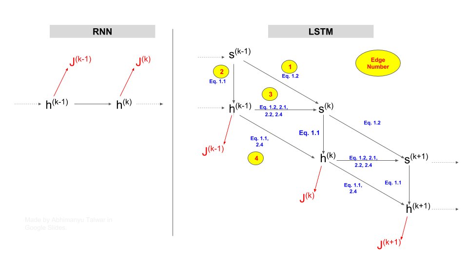
In the case of RNNs, given \(\gamma_{t}^{(k)}\), in order to calculate \(\gamma_{t}^{(k-1)}\), we only need to worry about the path between \(h^{(k-1)}\) and \(h^{(k)}\). That’s because any flow of influence between \(h^{(k-1)}\) and \(J^{(t)}\), must go through \(h^{(k)}\). Observe in the left column of the diagram below, that any path from \(h^{(k-1}\) to \(J^{(t)}\) (where \(t \geqslant k\)) must pass through \(h^{(k)}\).

The presence of a single node (\(h^{(k)}\)) through which all paths of influence from \(h^{(k-1)}\) to \(J^{(t)}\) must pass, is the reason our invariance involves a single quantity, which is \(\gamma_{t}^{(k)}\). This works slightly differently in the case of LSTMs.

In the diagram below, the influence of \(s^{(k-1)}\) on loss \(J^{(k)}\), flows via \(s^{(k)}\), through \(Edge \space 1\) and through \(Edges \space 2,3\). But observe that influence of \(s^{(k-1)}\) can also flow through a path comprising \(Edges \space 2,4\), and that this path bypasses \(s^{(k)}\) altogether!

In short, we need to consider ALL paths of influence! Our invariant for LSTMs has to include something in addition to \(\delta_{t}^{(k)}\). One candidate for that something is \(\gamma_{t}^{(k-1)}\).

Figure: Comparison of Paths of Influence in RNNs and LSTMs

This insight enables us to frame Claim 2, which is slightly different from what I had claimed for RNNs in my previous blog post.

Claim 2: At time-step \(k\), given \(\gamma_{t}^{(k-1)}\) and \(\delta_{t}^{(k)}\), we can compute \(\delta_{t}^{(k-1)}\) using only locally available information (i.e. information which was cached during the forward-pass through time-step \(k\)).

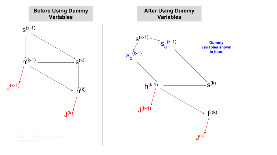
Proof: We want to capture all paths of influence between \(s^{(k-1)}\) and \(J^{(t)}\). But we also do not want to double-count any flow of influence! We are looking to combine the flow of influence of \(s^{(k-1)}\) via two paths: one through \(s^{(k)}\) and the other through \(h^{(k-1)}\). How do we combine these influences? Can we simply add them?

The answer is No. And that’s because there is some flow between these two paths via edge 3 in the diagram above. A way out of this to reuse our concept of ‘dummy variables’. We pretend that there are two versions of \(s^{(k-1)}\):

• \(s_{a}^{(k-1)}\), whose influence flows only via edge 1.
• \(s_{b}^{(k-1)}\), whose influence flows only via edges 2 and 3.

The figure below shows how paths of influence look like after applying ‘dummy variables’.

Figure: Isolating paths of influence via Dummy Variables

We can now express gradient w.r.t \(s^{(k-1)}\) as the sum of gradients w.r.t the dummy variables \(s_{a}^{(k-1)}\) and \(s_{a}^{(k-1)}\):

\[\frac {\partial J^{(t)}} {\partial s_{[i]}^{(k-1)}} = \underbrace{\frac {\partial J^{(t)}} {\partial s_{a[i]}^{(k-1)}}}_{\text{Eq. 7.0.1}} + \underbrace{\frac {\partial J^{(t)}} {\partial s_{b[i]}^{(k-1)}}}_{\text{Eq. 7.0.2}} \tag{7.0}\]

Let us consider the first path of influence:

\[\begin{align} \frac {\partial J^{(t)}} {\partial s_{a[i]}^{(k-1)}} &= \sum_{p=1}^{D} \frac {\partial J^{(t)}} {\partial s_{[p]}^{(k)}} \times \frac {\partial s_{[p]}^{(k)}} {\partial s_{a[i]}^{(k-1)}} \\[2ex] &= \delta_{t[i]}^{(k)} f^{(k)}_{[i]} \tag{7.0.1} \end{align}\]

And the second path of influence:

\[\begin{align} \frac {\partial J^{(t)}} {\partial s_{b[i]}^{(k-1)}} &= \sum_{p=1}^{D} \underbrace{\frac {\partial J^{(t)}} {\partial h_{[p]}^{(k-1)}}}_{\gamma_{[p]t}^{(k-1)}} \times \underbrace{\frac {\partial h_{[p]}^{(k-1)}} {\partial s_{b[i]}^{(k-1)}}}_{\text{Eq. 7.0.2.1}} \tag{7.0.2} \\[2ex] \end{align}\]

The first quantity on the right hand side is simply the \(p^{th}\) element of \(\gamma_{t}^{(k-1)}\). We can use \(Eq. 1.1\) to calculate the simple derivative required for the second quantity:

\[\frac {\partial h_{[p]}^{(k-1)}} {\partial s_{b[i]}^{(k-1)}} = \begin{cases} 0, & \text{p $\ne$ i} \\[2ex] q_{[i]}^{(k-1)} \times tanh'(s_{b[i]}^{(k-1)}), & \text{p = i} \tag{7.0.2.1} \end{cases}\]

Substituting this result in \(Eq. 7.0.2\), we get:

\[\frac {\partial J^{(t)}} {\partial s_{b[i]}^{(k-1)}} = \gamma_{t[i]}^{(k-1)} \times q_{[i]}^{(k-1)} \times tanh'(s_{b[i]}^{(k-1)})\]

Substituting \(Eq. 7.0.1\) and \(Eq. 7.0.2\) in \(Eq. 7.0\), we finally get:

\[\underbrace{\frac {\partial J^{(t)}} {\partial s_{[i]}^{(k-1)}}}_{\delta_{t[i]}^{(k-1)}} = \gamma_{t[i]}^{(k-1)} \times q_{[i]}^{(k-1)} \times tanh'(s_{[i]}^{(k-1)}) + \delta_{t[i]}^{(k)} \times f^{(k)}_{[i]}\]

Expressing this in matrix form:

\[\bbox[yellow,5px,border: 2px solid red] { \delta_{t}^{(k-1)} = \gamma_{t}^{(k-1)} \circ q^{(k-1)} \circ tanh'(s^{(k-1)}) + \delta_{t}^{(k)} \circ f^{(k)} \qquad (7.1) }\]

Let me take a moment to piece together what we’ve got so far:

1. In \(Eq. 6.2\), we derived an expression to calculate gradient of loss \(J^{(t)}\) in terms of locally available variables and one \(\delta_{t}^{(k)}\).
2. In \(Eq. 7.1\), we’ve derived a way to recursively calculated \(\delta_{t}^{(k-1)}\) using \(\delta_{t}^{(k)}\) and \(\gamma_{t}^{(k-1)}\) (which can also be computed in a similar recursive manner - see below).

Using \(Eq. 6.2\) and \(Eq. 7.1\) in conjunction, we should now be able to calculate gradient of \(J^{(t)}\) w.r.t \(W_{f}^{(k)}\).

We can derive a recursive expression for \(\gamma_{t}^{(k)}\) (i.e. \(\frac {\partial J^{(t)}} {\partial h^{(k-1)}}\)) in a manner similar to our derivation for \(\delta_{t}^{(k)}\) above. I provide the expression below (if you would like to know about its derivation, let me know via comments below).

\[\bbox[yellow,5px, border: 2px solid red] { \begin{align} \gamma_{t}^{(k-1)} &= (W_{f}^{(k)})^{Tr} \left( \delta_{t}^{(k)} \circ s^{(k-1)} \circ \sigma'(z_{f}^{(k)}) \right) \\[2ex] &+ (W_{e}^{(k)})^{Tr} \left( \delta_{t}^{(k)} \circ g^{(k)} \circ \sigma'(z_{e}^{(k)}) \right) \\[2ex] &+ (W_{g}^{(k)})^{Tr} \left( \delta_{t}^{(k)} \circ e^{(k)} \circ \sigma'(z_{g}^{(k)}) \right) \\[2ex] &+ (W_{q}^{(k)})^{Tr} \left( \gamma_{t}^{(k)} \circ tanh(s^{(k)}) \circ \sigma'(z_{q}^{(k)}) \right) \end{align} \qquad (8.1) }\]

Initial Conditions for Recursions: We have derived recursive expressions for \(\delta_{t}^{(k)}\) and \(\gamma_{t}^{(k)}\). Now we need to derive expressions for \(\delta_{t}^{(t)}\) and \(\gamma_{t}^{(t)}\) so that we can begin to apply \(Eq. 7.1\) and \(Eq. 8.1\) recursively. These are rather simple to compute.

The quantity \(h^{(t)}\) is connected to \(J^{(t)}\) via the Affine Layer followed by the Softmax Layer (see \(Eq. 3.0, \space 4.0, \space 4.0\)). We can compute \(\gamma_{t}^{(t)}\) by backpropogating through these layers.

Assuming we have calculated \(\gamma_{t}^{(t)}\), we apply chain-rule to get:

\[\begin{align} \underbrace{\frac {\partial J^{(t)}} {\partial s_{[i]}^{(t)}}}_{\delta_{t[i]}^{(t)}} &= \sum_{p=1}^{D} \frac {\partial J^{(t)}} {\partial h_{[p]}^{(t)}} \times \frac {\partial h_{[p]}^{(t)}} {\partial s_{[i]}^{(t)}} \\[2ex] &= \gamma_{t[i]}^{(t)} \times \underbrace{q_{[i]}^{(t)} \times tanh'(s_{[i]}^{(t)})}_{\text{Call it $c_{[i]}^{(t)}$}} \end{align}\]

In matrix notation:

\[\delta_{t}^{(t)} = \gamma_{t}^{(t)} \circ c^{(t)} \tag{9.0}\]

Accumulating Gradients for LSTMs

We now we have pretty much everything we need (in \(Eqs. 6.2, \space 7.1, \space 8.1\) and in the intial recursion conditions) to backprop through time for an LSTM and find gradients of \(J^{(t)}\) w.r.t \(W_{f}^{(k)}\) for \(k \in [0, t]\). But we need to do this for all values of \(t \in [0, T]\). This is where ‘accumulation of gradients’ will help us out.

At this point, I recommend you do not read any further unless you’ve looked at my post on RNNs where I describe how gradient accumulation works. If you’ve understood how gradient accumulation worked for RNNs, the following table will begin to make sense.

Let me explain what is happening at time-step \(T-1\), in this order:

We receive from time-step \(T\):

1. \(\gamma_{T}^{(T-1)}\), which was computed at step \(T\) using \(Eq. 8.1\)
2. \(f^{(T)} \circ \delta_{T}^{(T)}\), which was computed at step \(T\).

We compute at time-step \(T-1\):

1. \(\gamma_{T-1}^{(T-1)}\) and \(\delta_{T-1}^{(T-1)}\) using the Initial Recursion Conditions.
2. \(\gamma_{T-1}^{(T-2)}\) using \(Eq. 8.1\).
3. \(\delta_{T}^{(T-1)}\) using \(Eq. 7.1\).
4. \(\frac {\partial J^{(T-1)}} {\partial W_{f}^{(T-1)}}\) and \(\frac {\partial J^{(T-1)}} {\partial W_{f}^{(T-1)}}\) using \(Eq. 6.2\).

We pass on to time-step \(T-2\):

1. Sum of \(\gamma_{T-1}^{(T-2)}\) and \(\gamma_{T}^{(T-2)}\).
2. Sum of \(\left( f^{(T-1)} \circ \delta_{T-1}^{(T-1)} \right)\) and \(\left( f^{(T-1)} \circ \delta_{T}^{(T-1)} \right)\).

Note how we are passing sums of quantities (such as \(\gamma_{T-1}^{(T-2)}\) and \(\gamma_{T}^{(T-2)}\)) above instead of passing them individually. As I explained in detali in my post on RNN, this works because the equations which we are going to apply on these sums only contain Disitributive Operators (matrix multiplication and element-wise multiplication).

Table: Accumulation of \(\gamma_{t}^{(k)}\) and \(\delta_{t}^{(k)}\) for \(k \in [0,t], \space t \in [0,T]\)

\[\begin{array}{c|cc|cc|cc} \text{Time Step} & \text{At Current} & \text{Time Step} & \text{To Previous} & \text{Time Step} & \text{Gradients} & \text{Accumulated}\\ \hline T & \gamma_T^{(T)}, \delta_T^{(T)} & & \gamma_T^{(T-1)}, \left(f^{(T)} \circ \delta_T^{(T)}\right) & & \frac {\partial J^{(T)}} {\partial W_f^{(T)}} & \\[2ex] T-1 & \gamma_{T-1}^{(T-1)}, \delta_{T-1}^{(T-1)} & \gamma_{T}^{(T-1)}, \delta_{T}^{(T-1)} & \gamma_{T-1}^{(T-2)}, \left(f^{(T-1)} \circ \delta_{T-1}^{(T-1)}\right) & \gamma_{T}^{(T-2)}, \left(f^{(T-1)} \circ \delta_{T}^{(T-1)}\right) & \frac {\partial J^{(T-1)}} {\partial W_f^{(T-1)}} & \frac {\partial J^{(T)}} {\partial W_f^{(T-1)}} \\[2ex] \end{array}\]

Observe that in the last column of this Table, at each time-step \(k\) we are accumulating gradient of \(J^{(t)}\) w.r.t \(W_{f}^{(k)}\) for all \(t \in [k,\space k+1, \cdots, T-1, \space T]\).

Conclusion

The methodology of BPTT for an LSTM is very similar to that for an RNN. Although, I believe the calculation is more prone to mistakes stemming from incorrect application of the chain-rule. I did make those mistakes initially and learnt something from them, and then decided to put what I learnt into this blog post. I hope this helped you and if you spot any errors, please spell them out in the comments below or reach out to me via LinkedIn.