TL;DR

In this blog post:

1. I use SVD as a tool to explain what exactly \(L_2\) Regularization ‘does’ for Linear Regression.
2. The theory is borrowed from The Elements of Statistical Learning. What did I do?
   • I put the theory into practice with examples (all code available here).
   • I prove results which are not there or not clear in the book.

All Basis Vectors are not Equal

In the introductory last post on Singular Value Decomposition, I had demonstrated with examples how we can describe our data more efficiently with the help of SVD. In essence, instead of describing our data using the standard Cartesian Coordinate system, we instead used another Orthonormal Basis - the one given by the \(V\) matrix in the output of SVD. We saw how this particular Basis allowed us to convey a significant amount of information about data, by just using the first few Basis Vectors.

In other words, unlike the Cartesian Coordinate system, the SVD Orthonormal Basis comes with a heirarchy of Basis Vectors. Some Basis Vectors (such as the First Singular Vector) pack in a lot more information than the others. In this post, I will attempt to use this fact to gain more insight into Ridge Regression. The idea is borrowerd from Section 3.4.1 of the book The Elements of Statistical Learning by Hastie, Tibshirani, and Friedman. The book is incredibly densely packed with insights, and I highly recommend it.)

While you can always go to the book to view the key insights, in this post my aim is twofold:

• Demonstrate how those insights play out in practice with the help of real datasets.
• Provide detailed proofs of results which are not proved in the book, or for which the provided proofs are scant on details.

As with the previous post, I have created a companion python notebook which replicates the examples used in this post. Before we discuss Ridge Regression, let’s spend some more time on the ‘heirarchy’ of SVD Basis Vectors.

How do some Basis Vectors pack more information?

Say we have an \(m \times n\) matrix which represents \(m\) points in an \(n\)-dimensional space. We project each of these \(m\) points on to each vector in our ‘Best Fit’ Orthonormal Basis. So for each basis vector, we get a list of projection lengths of size \(m\) (one projection length for each point). When we calculate the sample variance of entries in such a projection length list, we will find that the variance is maximum for projections on the First Singular Vector. What this means intuitively is that the First Singular Vector is best able to ‘discern’ between all our \(m\) datapoints, among all Singular Vectors.”

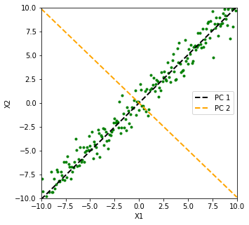
Toy Example for Intuition: Say we’ve been given 100 samples of two variables \(X_1\) and \(X_2\), which we need to use to build a prediction model for some quantity \(y\). But suppose we know that \(X_2\) is simply \(X_1\) plus some standard Gaussian noise. Clearly in this case there is no benefit to be received from using both \(X_1\) and \(X_2\) in our model - one of the two variables captures all the information that exists.

In the Figure below, we plot \(X_1\) vs. \(X_2\) (the green points), and we see that the First Singular Vector (the black line), points in the direction in which we are able to capture bulk of the variance between our 100 sample points. The Second Singular Vector (the orange line) only seems to be explaining variance due to the standard Gaussian noise. Intuitively, lengths of projections of the green points on our black line ‘vary a lot’, whereas their projections on the orange line seem to be contained within a narrow range of \([-1, 1]\), seemingly because of our standard Gaussian noise.

Figure 1: First Singular Vector (Black Line) Captures Direction of Maximum Variance

P.S. In an Appendix towards the end of this post , I will prove a result stated in ‘The Elements of Statistical Learning’ which will quantify the variance captured by any Singular Vector.

How does this relate to a Prediction Problem?

In a typical prediction problem, our task is to train a model which can predict some ‘target quantity’ (such as weight) or ‘target label’ (risk of heart attack - high, medium, or low), given values of ‘predictor’ variables (such as age, gender etc.). If we are able to discern between our ‘predictor’ variable samples, we will more clearly be able to ‘see’ the relationship between those variables and the ‘target’.

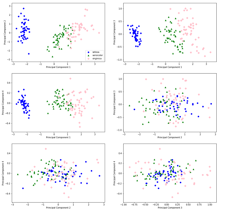
Let us understand this with the help of the Iris dataset in which we are given 150 samples of four Predictor variables - the lengths and widths of sepals and petals - and we need to classify a sample into one of three species of Iris (Setosa, Virginica, and Versicolor).

In the Figure below, for each subplot, we choose two Basis Vectors from our set of four Singular Vectors, and plot the projection of our sample data matrix, onto this subspace comprising those two Basis Vectors.

Hands down, the First Principal Component (which captures the maximum variance within the ‘predictor’ variable samples in our dataset) is able to discern between the three Iris categories better than any other Principal Component! In the first three subplots, you can simply eyeball the figures and come up with ranges for the value of ‘Principal Component 1’, which can form a good indicator of the Iris species. For instance, by looking at the first plot, we can say that if the value of Principal Component 1 for an Iris sample is less than \(-1\), it is likely that it belongs to the ‘Setosa’ species.

Figure 2: Principal Component 1 Packs the Maximum Info!

Ridge Regression

Armed with some intuition into how Singular Vectors capture variance within a set of points, let us now apply that to analyzing Ridge Regression.

Linear Regression Basics

In Linear Regression, we assume that a linear relationship exists between our target variable (i.e. the quantity we are trying to predict) \(y\) (where \(y \in \mathbb{R}\)) and our predictor variable(s) \(x_1, \space \cdots, \space x_n\) (where each \(x_i \in \mathbb{R}, \text{for } i \in [1, \cdots, n]\)). We say that this relationship is ‘parametrized’ by a quantity \(\beta \in \mathbb{R}^n\) i.e. \(\beta = (\beta_1, \cdots, \beta_n)\), which we do not know. This relationship can be written as:

\[y = x^{T}\beta\]

Note: Throughout this post we assume each vector is a column vector. Hence, in the equation above, \(\beta\) is a column vectors and so I have matrix-multiplied transpose of \(x\).

We do not know the parameter \(\beta\), but we can estimate it from samples \([(y^{(1)}, x^{(1)}), \cdots, (y^{(m)}, x^{(m)})]\). One way to find this estimate is to find a vector \(\beta\) which minimizes the squared sum of ‘errors’. This minimization problem is stated as:

\[\text{Minimize}_{\beta \in \mathbb{R}^n} \space \underbrace{\sum_{j=1}^{m} (\underbrace{y^{(j)} - (x^{(j)})^{T}\beta}_{\text{Error for $j^{th}$ sample}})^2}_{\text{The Objective Function}}\]

This can be stated in matrix notations as:

\[\text{Minimize}_{\beta \in \mathbb{R}^{n}} \space (Y - X\beta)^{T}(Y - X\beta)\]

Note: Here, \(Y\) is a vector of dimensions \((m \times 1)\), \(X\) is a matrix of dimensions \((m \times n)\), and \(\beta\) is a vector of dimensions \(n \times 1\).

This is a convex optimization problem, and its solution (i.e. the value of \(\beta\) which minimizes the sum of squared erors) can be found analytically:

\[\hat{\beta} = (X^{T}X)^{-1}X^{T}y \tag{1}\]

Note: One can see from \(Eq. 1\) that this solution exists only when the matrix \((X^{T}X)\) is invertible. For this to hold true, it is enough that \(X\) has full column rank (see Appendix below for my proof). If you do not understand this Note, it is okay, and for now just assume that the solution in \(Eq. 1\) exists.

From Linear Regression to Ridge Regression

We are trying to solve the same prediction problem as we were for Linear Regression above, i.e. we assume that a linear relationship exists between \(y\) and \(x \in \mathbb{R}^{n}\) parametrized by some \(\beta \in \mathbb{R}^{n}\), which we are trying to estimate from \(m\) samples. When doing Ridge Regression we introduce a slight tweak to the Objecive Function - the optimization problem now is:

\[\text{Minimize}_{\beta \in \mathbb{R}^{n}} (Y - X\beta)^{T}(Y - X\beta) + \lambda\beta^{T}\beta \qquad{(\lambda \in \mathbb{R}^{+})}\]

Now we are trying to minimize the sum of (1) sum of squared errors, and (2) square of length of our parameter vector. Intuitively, we are saying that we want to find a \(\beta\) which reduces the sum of squared errors, but which is itself not too large a vector. We express our preference for how ‘small’ we want \(\beta\) to be through our choice of the ‘hyperparamter’ \(\lambda\).

But why do we want a ‘small’ \(\beta\) vector? How does this small \(\beta\) differ from what we get from Linear Regression in \(Eq. 1\)? Answering these questions is the goal of this blog post, and SVD is going to help us gain some insights.

As it turns out, Ridge Regression also has an analytical solution given by:

\[\hat{\beta}^{Ridge} = (X^{T}X + \lambda I)^{-1}X^{T}y \tag{2}\]

Note: This solution in \(Eq. 2\) always exists for \(\lambda > 0\) - see Appendix for a simple proof.

Using SVD to Gain Insights into Ridge Regression

Let me get started by restating the magic result from Section 3.4.1 of The Elements of Statistical Learning:

\[\bbox[yellow,5px,border:2px solid red] { X\hat{\beta}^{Ridge} = \sum_{j=1}^{p} u_j \frac {d_j^{2}}{d_j^{2} + \lambda} u_j^{T}y \qquad (3) }\]

Note: This result is proved in the book in three lines, however I am going to elaborate on the proof in Appendix (1) below so that every intermediate step which is not in the book is clear to the reader.

To understand this magic result, let’s see what this implies for the case of simple Linear Regression (i.e. when \(\lambda \space = \space 0\)):

\[\begin{align} \hat{y} &= X\hat{\beta}^{Ridge} \\ &= \sum_{j=1}^{p} \underbrace{(u_j^{T}y)}_{\substack{\text{Length of} \\ \text{projection of} \\ \text{y on $u_j$}}} \times \underbrace{u_j}_{\substack{\text{A unit} \\ \text{vector}}}\\[2ex] \tag{4} &= \sum_{j=1}^{p} \text{Projection of $y$ on $u_j$} \end{align}\]

According to \(Eq. 4\), our model’s ‘predictions’ \(\hat{y}\) are the sum of projections of the ‘truth’ \(y\) on each of the Left Singular Vectors (the \(u_j\)s). Now if \(\lambda > 0\), then using \(Eq. 3\) and \(Eq. 4\), we have:

\[\begin{align} \hat{y} &= \sum_{j=1}^{p} \text{Projection of $y$ on $u_j$} \times \underbrace{\frac {d^{2}_{j}} {d^{2}_{j} + \lambda}}_{\substack{\text{Scaledown} \\ \text{Factor}}} \end{align}\]

How much does the Scaledown Factor scales down projections of \(y\) on each \(u_j\)? That depends on the magnitude of the corresponding Singular Value \(d_{j}\). The Figure below plots Scaledown Factor versus square of corresponding Singular Value.

Figure 3: Scaledown Factor vs Squared Singular Value

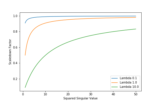
The Figure shows that the Scaledown Factor approaches \(1.0\) for large Singular Values, irrespective of the value of \(\lambda\). Observe that for the same value of \(\lambda\), projections of \(y\) on basis vectors with small Singular Values will be scaled down relative to projections on basis vector with large Singular Values. Moreover, higher the value of \(\lambda\), stronger is this Scale Down effect.

Appendix:

(1) Detailed proof of the ‘magic result’ from The Elements of Statistical Learning

Using SVD, we can factor \(X\) as follows:

\[X = U \space D \space V^{T} \tag{5}\]

We will replace \(X\) with its SVD factorization in \(Eq. 1\). Let’s also calculate \((X^{T}X)\):

\[\begin{align} X^{T}X &= (UDV^{T})^{T}(UDV^{T})\\[2ex] &= (V\underbrace{\space \space D^{T} \space \space}_{\text{Equals } D \space \because \space D \text{ is diagonal}}U^{T})(UDV^{T})\\[2ex] &= VD\underbrace{\space U^{T}U \space}_{\substack{\text{Equals I} \\ \text{$\because$ U is} \\ \text{Orthonormal}}}DV^{T}\\[2ex] &= VD^{2}V^{T} \tag{6} \end{align}\]

Using \(Eq. 5\) and \(Eq. 6\) in \(Eq. 2\):

\[\begin{align} \hat{\beta}^{Ridge} &= (VD^{2}V^{T} + \lambda\underbrace{I}_{\text{Replace I with $VV^{T}$}})^{-1}\underbrace{(UDV^{T})^{T}}_{\text{Equal $VDU^{T}$}}y\\[2ex] &= (VD^{2}V^{T} + \lambda VV^{T})^{-1}VDU^{T}y\\[2ex] &= (V(D^{2} + \lambda I)V^{T})^{-1}VDU^{T}y \end{align}\]

Now we use the fact that for matrices \(A\), \(B\), and \(C\):

\[(ABC)^{-1} = C^{-1}B^{-1}A^{-1}\] \[\begin{align} \therefore \hat{\beta}^{Ridge} &= \underbrace{(V^{T})^{-1}}_{\substack{\text{Equals V} \\ \text{$\because \space V^{T}V = I$}}}(D^{2} + \lambda I)^{-1}\underbrace{V^{-1}V}_{\text{Equals I}}DU^{T}y\\[2ex] &= V(D^{2} + \lambda I)^{-1}DU^{T}y\\[2ex] \tag{7} \end{align}\]

Now our model’s predictions are:

\[\begin{align} X\hat{\beta}^{Ridge} &= \underbrace{XV}_{\text{Equals UD}}(D^{2} + \lambda I)^{-1}DU^{T}y\\[2ex] &= UD(D^{2} + \lambda I)^{-1}DU^{T}y \tag{8} \end{align}\]

\(Eq. 3\) is just an expanded form of \(Eq. 8\) above. Hence proved.

(2) If \(\lambda > 0\), the matrix \(X^{T}X + \lambda I\) is always invertible

To show that the matrix \(X^{T}X + \lambda I\) is invertible for \(\lambda > 0\), it suffices to show that this matrix is Positive Definite under the constraint on \(\lambda\). A matrix \(A\) is Positive Definite if \(y^{T}Ay\) is strictly positive \(\forall y \ne 0\).

\[\begin{align} y^{T}(X^{T}X + \lambda I)y &= y^{T}X^{T}Xy + \lambda y^{T}y\\[2ex] &= \underbrace{(Xy)^{T}(Xy)}_{\geqslant 0} + \underbrace{\space \lambda y^{T}y \space}_{>0 \text{ for } \lambda > 0, \space y \ne 0}\\[2ex] &> 0 \end{align}\]

(3) If \(X\) has full column rank, \((X^{T}X)\) is invertible

Consider the scalar quantity \(y^{T}(X^{T}X)y\). It can be written as \((Xy)^{T}(Xy)\). Written this way, it now represents the squared length of the vector \(Xy\). This squared length is non-negative for sure.

If matrix \(X\) has full-column rank, then its Null Space only contains the zero vector. This implies that squared length of vector \(Xy\) is always greater than 0 \(\forall y > 0\). In other words, the matrix \(X\) is Positive Definite and therefore invertible.

Quantifying the Variance captured by a Singular Vector

Coming soon.